


Introduction to Artificial Neural Networks in Python
Table of Contents
- Biology inspires the Artificial Neural Network
- What is an Artificial Neural Network?
- Perceptron model
- Training phase of a neural network
- Bringing it all together
- Conclusion
The Python implementation presented may be found in the Kite repository on Github.
Biology inspires the Artificial Neural Network
The Artificial Neural Network (ANN) is an attempt at modeling the information processing capabilities of the biological nervous system. The human body is made up of trillions of cells, and the nervous system cells – called neurons – are specialized to carry “messages” through an electrochemical process. The nodes in ANN are equivalent to those of our neurons, whose nodes are connected to each other by Synaptic Weights (or simply weights) – equivalent to the synaptic connections between axons and dendrites of the biological neuron.

Let’s think of a scenario where you’re teaching a toddler how to identify different kinds of animals. You know that they can’t simply identify any animal using basic characteristics like a color range and a pattern: just because an animal is within a range of colors and has black vertical stripes and a slightly elliptical shape doesn’t automatically make it a tiger.
Instead, you should show them many different pictures, and then teach the toddler to identify those features in the picture on their own, hopefully without much of a conscious effort. This specific ability of the human brain to identify features and memorize associations is what inspired the emergence of ANNs.
What is an Artificial Neural Network?
In simple terms, an artificial neural network is a set of connected input and output units in which each connection has an associated weight. During the learning phase, the network learns by adjusting the weights in order to be able to predict the correct class label of the input tuples. Neural network learning is also referred to as connectionist learning, referencing the connections between the nodes. In order to fully understand how the artificial neural networks work, let’s first look at some early design approaches.
What can an Artificial Neural Network do?
Today, instead of designing a standardized solutions to general problems, we focus on providing a personalized, customized solution to specific situations. For instance, when you log in to any e-commerce website, it’ll provide you with personalized product recommendations based on your previous purchase, items on your wishlist, most frequently clicked items, and so on.
The platform is essentially analyzing the user’s behavior pattern and then recommending the solution accordingly; solutions like these can be effectively designed using Artificial Neural Networks.
ANNs have been successfully applied in wide range of domains such as:
- Classification of data – Is this flower a rose or tulip?
- Anomaly detection – Is the particular user activity on the website a potential fraudulent behavior?
- Speech recognition – Hey Siri! Can you tell me a joke?
- Audio generation – Jukedeck, can you compose an uplifting folk song?
- Time series analysis – Is it good time to start investing in stock market?
And the list goes on…
Early model of ANN
The McCulloch-Pitts model of Neuron (1943 model)
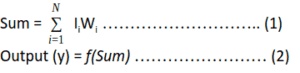
This model is made up of a basic unit called Neuron. The main feature of their Neuron model is that a weighted sum of input signals is compared against a threshold to determine the neuron output. When the sum is greater than or equal to the threshold, the output is 1. When the sum is less than the threshold, the output is 0. It can be put into the equations as such:
This function f which is also referred to as an activation function or transfer function is depicted in the figure below, where T stands for the threshold.
The figure below depicts the overall McCulloch-Pitts Model of Neuron.
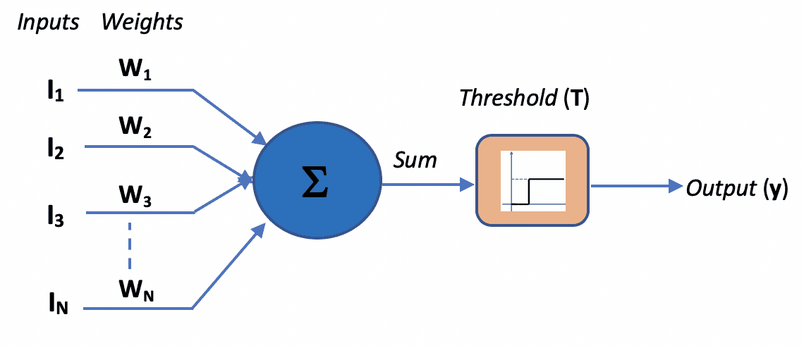
Let’s start by designing the simplest Artificial Neural Network that can mimic the basic logic gates. On the left side, you can see the mathematical implementation of a basic logic gate, and on the right-side, the same logic is implemented by allocating appropriate weights to the neural network.
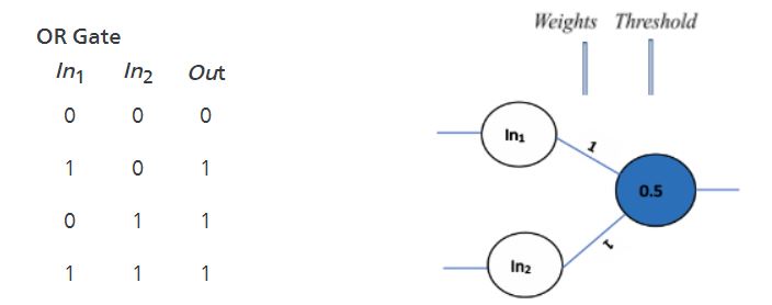
If you give the first set of inputs to the network i.e. (0, 0) it gets multiplied by the weights of the network to get the sum as follows: (0*1) + (0*1) = 0 (refer eq. 1). Here, the sum, 0, is less than the threshold, 0.5, hence the output will be 0 (refer eq. 2).
Whereas, for the second set of inputs (1,0), the sum (1*1) + (0*1) = 1 is greater than the threshold, 0.5, hence the output will be 1.
Similarly, you can try any different combination of weights and thresholds to design the neural network depicting AND gate and NOT gate as shown below.
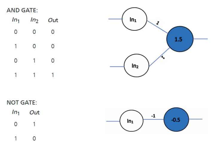
This way, the McCulloch-Pitts model demonstrates that networks of these neurons could, in principle, compute any arithmetic or logical function.
Perceptron model
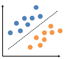
This is the simplest type of neural network that helps with linear (or binary) classifications of data. The figure below shows the linearly separable data.
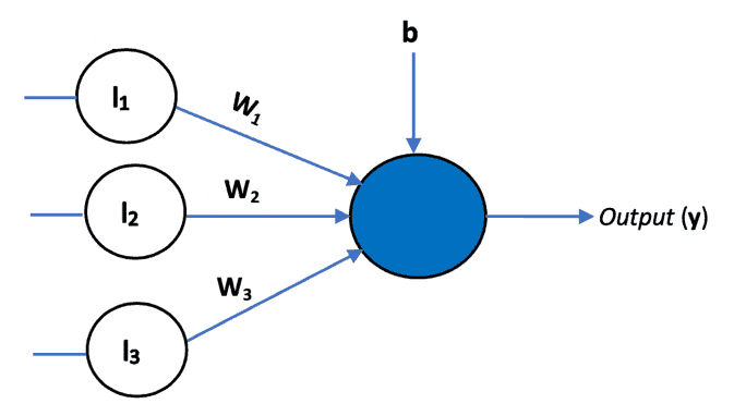
The learning rule for training the neural network was first introduced with this model. In addition to the variable weight values, the perceptron added an extra input that represents bias. Thus, the equation 1 was modified as follows:
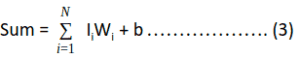
Bias is used to adjust the output of the neuron along with the weighted sum of the inputs. It’s just like the intercept added in a linear equation.
Multilayer perceptron model
A perceptron that as a single layer of weights can only help in linear or binary data classifications. What if the input data is not linearly separable, as shown in figure below?
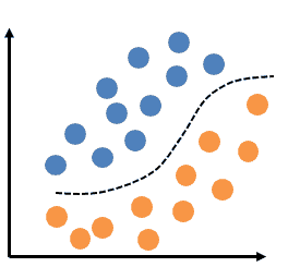
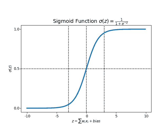
This is when we use a multilayer perceptron with a non-linear activation function such as sigmoid.
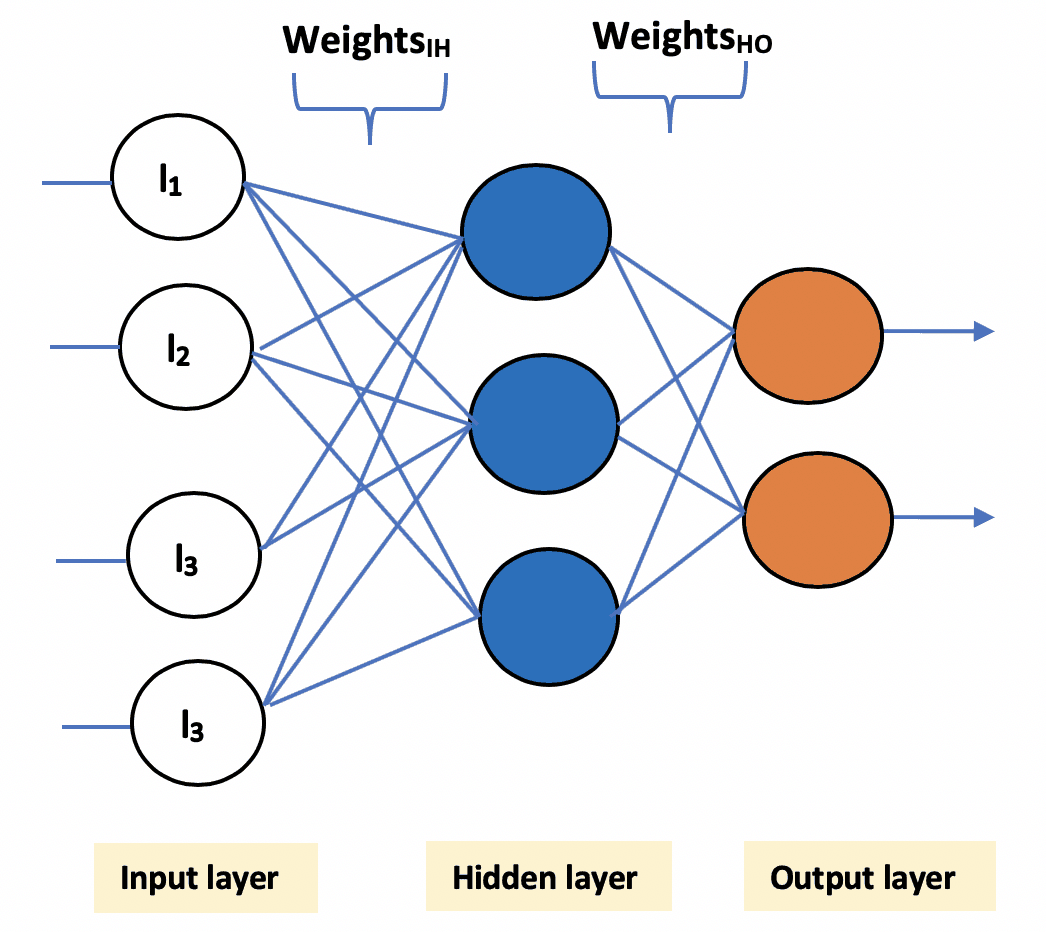
Multilayer perceptron has three main components:
- Input layer: This layer accepts the input features. Note that this layer does not perform any computation – it just passes on the input data (features) to the hidden layer.
- Hidden layer: This layer performs all sorts of computations on the input features and transfers the result to the output layer. There can be one or more hidden layers.
- Output layer: This layer is responsible for producing the final result of the model.
Now that we’ve discussed the basic architecture of a neural network, let’s understand how these networks are trained.
Training phase of a neural network
Training a neural network is quite similar to teaching a toddler how to walk. In the beginning, when she is first trying to learn, she’ll naturally make mistakes as she learns to stand on her feet and walk gracefully.
Similarly, in the initial phase of training, neural networks tend to make a lot of mistakes. Initially, the predicted output could be stunningly different from the expected output. This difference in predicted and expected outputs is termed as an ‘error’.
The entire goal of training a neural network is to minimize this error by adjusting its weights.
This training process consists of three (broad) steps:
1. Initialize the weights
The weights in the network are initialized to small random numbers (e.g., ranging from -1 to 1, or -0.5 to 0.5). Each unit has a bias associated with it, and the biases are similarly initialized to small random numbers.
def initialize_weights():

    # Generate random numbers

    random.seed(1)


    # Assign random weights to a 3 x 1 matrix

    synaptic_weights = random.uniform(low=-1, high=1, size=(3, 1))

    return synaptic_weights
2. Propagate the input forward
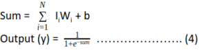
In this step, the weighted sum of input values is calculated, and the result is passed to an activation function – say, a sigmoid activation function – which squeezes the sum value to a particular range (in this case, between 0 to 1), further adding bias with it. This decides whether a neuron should be activated or not.
Our sigmoid utility functions are defined like so:
def sigmoid(x):

    return 1 / (1 + exp(-x))


def sigmoid_derivative(x):

    return x * (1 - x)
3. Backpropagate the error
In this step, we first calculate the error, i.e., the difference between our predicted output and expected output. Further, the weights of the network are adjusted in such a way that during the next pass, the predicted output is much closer to the expected output, thereby reducing the error.
For neuron j (also referred to as unit j) of the output layer, the error is computed as follows:
Errj = Oj*(1 – Oj )*( Tj – Oj ) ……………….. (5)Where Tj is the expected output, Oj is the predicted output and Oj *(1 – Oj) is the derivative of sigmoid function.
The weights and biases are updated to reflect the back propagated error.
Wij = Wij + (l*Errij*Oj ) ………………………. (6)

bi = bj + (l* Errij) ……………………………….  (7)
Above, l is the learning rate, a constant typically varying between 0 to 1. It decides the rate at which the value of weights and bias should vary. If the learning rate is high, then the weights and bias will vary drastically with each epoch. If it’s too low, then the change will be very slow.
We terminate the training process when our model’s predicted output is almost same as the expected output. Steps 2 and 3 are repeated until one of the following terminating conditions is met:
- The error is minimized to the least possible value
- The training has gone through the maximum number of iterations
- There is no further reduction in error value
- The training error is almost same as that of validation error
So, let’s create a simple interface that allows us to run the training process:
def learn(inputs, synaptic_weights, bias):

     return sigmoid(dot(inputs, synaptic_weights) + bias)


def train(inputs, expected_output, synaptic_weights, bias, learning_rate, training_iterations):

     for epoch in range(training_iterations):

          # Forward pass -- Pass the training set through the network.

          predicted_output = learn(inputs, synaptic_weights, bias)


        # Backaward pass

        # Calculate the error

        error = sigmoid_derivative(predicted_output) * (expected_output - predicted_output)


        # Adjust the weights and bias by a factor

        weight_factor = dot(inputs.T, error) * learning_rate

        bias_factor = error * learning_rate


        # Update the synaptic weights

        synaptic_weights += weight_factor


        # Update the bias

        bias += bias_factor


        if ((epoch % 1000) == 0):

            print("Epoch", epoch)

            print("Predicted Output = ", predicted_output.T)

            print("Expected Output = ", expected_output.T)

            print()

    return synaptic_weights
Bringing it all together
Finally, we can train the network and see the results using the simple interface created above. You’ll find the complete code in the Kite repository.
# Initialize random weights for the network

    synaptic_weights = initialize_weights()


    # The training set

    inputs = array([[0, 1, 1],

                    [1, 0, 0],

                    [1, 0, 1]])


    # Target set

    expected_output = array([[1, 0, 1]]).T


    # Test set

    test = array([1, 0, 1])


    # Train the neural network

    trained_weights = train(inputs, expected_output, synaptic_weights, bias=0.001, learning_rate=0.98,

                            training_iterations=1000000)


    # Test the neural network with a test example

    accuracy = (learn(test, trained_weights, bias=0.01)) * 100


    print("accuracy =", accuracy[0], "%")
Conclusion
You now have seen a sneak peek into Artificial Neural Networks! Although the mathematics behind training a neural network might have seemed a little intimidating at the beginning, you can now see how easy it is to implement them using Python.
In this post, we’ve learned some of the fundamental correlations between the logic gates and the basic neural network. We’ve also looked into the Perceptron model and the different components of a multilayer perceptron.
In my upcoming post, I’m going to talk about different types of artificial neural networks and how they can be used in your day-to-day applications. Python is well known for its rich set of libraries like Keras, Scikit-learn, and Pandas to name a few – which abstracts out the intricacies involved in data manipulation, model building, training the model, etc. We shall be seeing how to use these libraries to build some of the cool applications. This post is an introduction to some of the basic concepts involved in building these models before we dive into using libraries.
Try it yourself
The best way of learning is by trying it out on your own, so here are some questions you can try answering using the concepts we learned in this post:
- Can you build an XOR model by tweaking the weights and thresholds?
- Try adding more than one hidden layer to the neural network, and see how the training phase changes.
See you in the next post!
Resources
 in San Francisco