Image Segmentation with Python
Table of Contents
- Introduction to image segmentation
- Approach
- Loading and visualizing data
- Pre-processing
- Segmentation
- Validation
- Validation visualization
- Final notes
Introduction to image segmentation
In this article we look at an interesting data problem – making decisions about the algorithms used for image segmentation, or separating one qualitatively different part of an image from another.
Example code for this article may be found at the Kite Github repository. We have provided tips on how to use the code throughout.
As our example, we work through the process of differentiating vascular tissue in images, produced by Knife-edge Scanning Microscopy (KESM). While this may seem like a specialized use-case, there are far-reaching implications, especially regarding preparatory steps for statistical analysis and machine learning.
Data scientists and medical researchers alike could use this approach as a template for any complex, image-based data set (such as astronomical data), or even large sets of non-image data. After all, images are ultimately matrices of values, and we’re lucky to have an expert-sorted data set to use as ground truth. In this process, we’re going to expose and describe several tools available via image processing and scientific Python packages (opencv, scikit-image, and scikit-learn). We’ll also make heavy use of the numpy library to ensure consistent storage of values in memory.
The procedures we’ll explore could be used for any number of statistical or supervised machine learning problems, as there are a large number of ground truth data points. In order to choose our image segmentation algorithm and approach, we will demonstrate how to visualize the confusion matrix, using matplotlib to colorize where the algorithm was right and where it was wrong. In early stages, it’s more useful for a human to be able to clearly visualize the results than to aggregate them into a few abstract numerals.
Approach
Cleaning
To remove noise, we use a simple median filter to remove the outliers, but one can use a different noise removal approach or artifact removal approach. The artifacts vary across acquisition systems (microscopy techniques) and may require complicated algorithms to restore the missing data. Artifacts commonly fall into two categories:
- blurry or out-of-focus areas
- imbalanced foreground and background (correct with histogram modification)
Segmentation
For this article, we limit segmentation to Otsu’s approach, after smoothing an image using a median filter, followed by validation of results. You can use the same validation approach for any segmentation algorithm, as long as the segmentation result is binary. These algorithms include, but are not limited to, various Circular Thresholding approaches that consider different color space.
Some examples are:
- Li Thresholding
- An adaptive thresholding method that is dependent on local intensity
- Deep learning algorithms like UNet used commonly in biomedical image segmentation
- Deep learning approaches that semantically segment an image
Validation
We begin with a ground truth data set, which has already been manually segmented. To quantify the performance of a segmentation algorithm, we compare ground truth with the predicted binary segmentation, showing accuracy alongside more effective metrics. Accuracy can be abnormally high despite a low number of true positives (TP) or false negatives (FN). In such cases, F1 Score and MCC are better quantification metrics for the binary classification.We’ll go into detail on the pros and cons of these metrics later.
For qualitative validation, we overlay the confusion matrix results i.e where exactly the true positives, true negatives, false positives, false negatives pixels are onto the grayscale image. This validation can also be applied to a color image on a binary image segmentation result, although the data we used in this article is a grayscale image. In the end, we will present the whole process so that you can see the results for yourself. Now, let’s look at the data–and the tools used to process that data.
Loading and visualizing data
We will use the below modules to load, visualize, and transform the data. These are useful for image processing and computer vision algorithms, with simple and complex array mathematics. The module names in parentheses will help if installing individually.
| Module | Reason |
| numpy | Histogram calculation, array math, and equality testing |
| matplotlib | Graph plotting and Image visualization |
| scipy | Image reading and median filter |
| cv2 (opencv-python) | Alpha compositing to combine two images |
| skimage (scikit-image) | Image thresholding |
| sklearn (scikit-learn) | Binary classifier confusion matrix |
| nose | Testing |
Displaying Plots Sidebar: If you are running the example code in sections from the command line, or experience issues with the matplotlib backend, disable interactive mode by removing the plt.ion() call, and instead call plt.show() at the end of each section, by uncommenting suggested calls in the example code. Either ‘Agg’ or ‘TkAgg’ will serve as a backend for image display. Plots will be displayed as they appear in the article.
Importing modules
import cv2

import matplotlib.pyplot as plt

import numpy as np

import scipy.misc

import scipy.ndimage

import skimage.filters

import sklearn.metrics


# Turn on interactive mode. Turn off with plt.ioff()

plt.ion()
In this section, we load and visualize the data. The data is an image of mouse brain tissue stained with India ink, generated by Knife-Edge Scanning Microscopy (KESM). This 512 x 512 image is a subset, referred to as a tile. The full data set is 17480 x 8026 pixels, 799 slices in depth, and 10gb in size. So, we will write algorithms to process the tile of size 512 x 512 which is only 150 KB.
Individual tiles can be mapped to run on multi processing/multi threaded (i.e. distributed infrastructure), and then stitched back together to obtain the full segmented image. The specific stitching method is not demonstrated here. Briefly, stitching involves indexing the full matrix and putting the tiles back together according to this index. For combining numerical values, you can use map-reduce. Map-Reduce yields metrics such as the sum of all the F1 scores along all tiles, which you can then average. Simply append the results to a list, and then perform your own statistical summary.
The dark circular/elliptical disks on the left are vessels and the rest is the tissue. So, our two classes in this dataset are:
- foreground (vessels) – labeled as 255
- background (tissue) – labeled as 0
The last image on the right below is the ground truth image. Vessels are traced manually by drawing up contours and filling them to obtain the ground truth by a board-certified pathologist. We can use several examples like these from experts to train supervised deep learning networks and validate them on a larger scale. We can also augment the data by giving these examples to crowdsourced platforms and training them to manually trace a different set of images on a larger scale for validation and training. The image in the middle is just an inverted grayscale image, which corresponds with the ground truth binary image.
Loading and visualizing images in figure above
grayscale = scipy.misc.imread('grayscale.png')

grayscale = 255 - grayscale

groundtruth = scipy.misc.imread('groundtruth.png')

plt.subplot(1, 3, 1)

plt.imshow(255 - grayscale, cmap='gray')

plt.title('grayscale')

plt.axis('off')

plt.subplot(1, 3, 2)

plt.imshow(grayscale, cmap='gray')

plt.title('inverted grayscale')

plt.axis('off')

plt.subplot(1, 3, 3)

plt.imshow(groundtruth, cmap='gray')

plt.title('groundtruth binary')

plt.axis('off')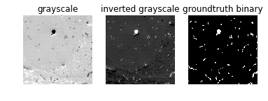
Pre-processing
Before segmenting the data, you should go through the dataset thoroughly to determine if there are any artifacts due to the imaging system. In this example, we only have one image in question. By looking at the image, we can see that there aren’t any noticeable artifacts that would interfere with the segmentation. However, you can remove outlier noise and smooth an image using a median filter. A median filter replaces the outliers with the median (within a kernel of a given size).
Median filter of kernel size 3
median_filtered = scipy.ndimage.median_filter(grayscale, size=3)

plt.imshow(median_filtered, cmap='gray')

plt.axis('off')

plt.title('median filtered image')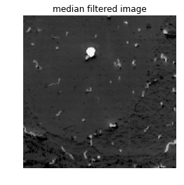
To determine which thresholding technique is best for segmentation, you could start by thresholding to determine if there is a distinct pixel intensity that separates the two classes. In such cases, you can use that intensity obtained by the visual inspection to binarize the image. In our case, there seem to be a lot of pixels with intensities of less than 50 which correspond to the background class in the inverted grayscale image.
Although the distribution of the classes is not bimodal (having two distinct peaks), it still has a distinction between foreground and background, which is where the lower intensity pixels peak and then hit a valley. This exact value can be obtained by various thresholding techniques. The segmentation section examines one such method in detail.
Visualize histogram of the pixel intensities
counts, vals = np.histogram(grayscale, bins=range(2 ** 8))

plt.plot(range(0, (2 ** 8) - 1), counts)

plt.title('Grayscale image histogram')

plt.xlabel('Pixel intensity')

plt.ylabel('Count')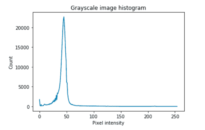
Segmentation
After removing noise, you can apply the skimage filters module to try all thresholds to explore which thresholding methods fare well. Sometimes, in an image, a histogram of its pixel intensities is not bimodal. So, there might be another thresholding method that can fare better like an adaptive thresholding method that does thresholding based on local pixel intensities within a kernel shape. It’s good to see what the different thresholding methods results are, and skimage.filters.thresholding.try_all_threshold() is handy for that.
Try all thresholding method
result = skimage.filters.thresholding.try_all_threshold(median_filtered)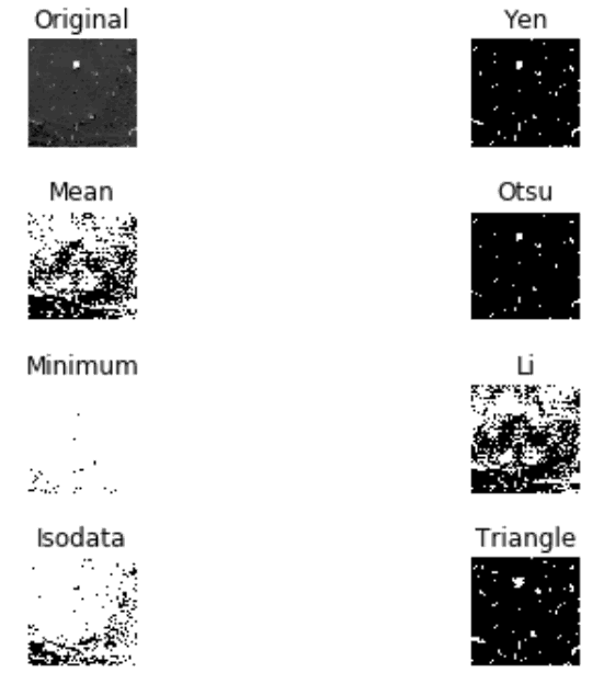
The simplest thresholding approach uses a manually set threshold for an image. On the other hand, using an automated threshold method on an image calculates its numerical value better than the human eye and may be easily replicated. For our image in this example, it seems like Otsu, Yen, and the Triangle method are performing well. The other results for this case are noticeably worse.
We’ll use the Otsu thresholding to segment our image into a binary image for this article. Otsu calculates thresholds by calculating a value that maximizes inter-class variance (variance between foreground and background) and minimizes intra-class variance (variance within foreground or variance within background). It does well if there is either a bimodal histogram (with two distinct peaks) or a threshold value that separates classes better.
Otsu thresholding and visualization
threshold = skimage.filters.threshold_otsu(median_filtered)

print('Threshold value is {}'.format(threshold))

predicted = np.uint8(median_filtered > threshold) * 255

plt.imshow(predicted, cmap='gray')

plt.axis('off')

plt.title('otsu predicted binary image')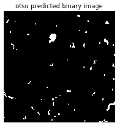
If the above simple techniques don’t serve the purpose for binary segmentation of the image, then one can use UNet, ResNet with FCN or various other supervised deep learning techniques to segment the images. To remove small objects due to the segmented foreground noise, you may also consider trying skimage.morphology.remove_objects().
Validation
In any of the cases, we need the ground truth to be manually generated by a human with expertise in the image type to validate the accuracy and other metrics to see how well the image is segmented.
The confusion matrix
We use sklearn.metrics.confusion_matrix() to get the confusion matrix elements as shown below. Scikit-learn confusion matrix function returns 4 elements of the confusion matrix, given that the input is a list of elements with binary elements. For edge cases where everything is one binary value(0) or other(1), sklearn returns only one element. We wrap the sklearn confusion matrix function and write our own with these edge cases covered as below:
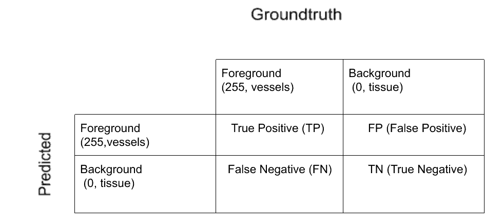
get_confusion_matrix_elements()
def get_confusion_matrix_elements(groundtruth_list, predicted_list):

    """returns confusion matrix elements i.e TN, FP, FN, TP as floats

	See example code for helper function definitions

    """

    _assert_valid_lists(groundtruth_list, predicted_list)


    if _all_class_1_predicted_as_class_1(groundtruth_list, predicted_list) is True:

        tn, fp, fn, tp = 0, 0, 0, np.float64(len(groundtruth_list))


    elif _all_class_0_predicted_as_class_0(groundtruth_list, predicted_list) is True:

        tn, fp, fn, tp = np.float64(len(groundtruth_list)), 0, 0, 0


    else:

        tn, fp, fn, tp = sklearn.metrics.confusion_matrix(groundtruth_list, predicted_list).ravel()

        tn, fp, fn, tp = np.float64(tn), np.float64(fp), np.float64(fn), np.float64(tp)


    return tn, fp, fn, tp
Accuracy
Accuracy is a common validation metric in case of binary classification. It is calculated as

where TP = True Positive, TN = True Negative, FP = False Positive, FN = False Negative
get_accuracy()
def get_accuracy(groundtruth_list, predicted_list):


    tn, fp, fn, tp = get_confusion_matrix_elements(groundtruth_list, predicted_list)


    total = tp + fp + fn + tn

    accuracy = (tp + tn) / total


    return accuracy
It varies between 0 to 1, with 0 being the worst and 1 being the best. If an algorithm detects everything as either entirely background or foreground, there would still be a high accuracy. Hence we need a metric that considers the imbalance in class count. Especially since the current image has more foreground pixels(class 1) than background 0.
F1 score
The F1 score varies from 0 to 1 and is calculated as:

with 0 being the worst and 1 being the best prediction. Now let’s handle F1 score calculation considering edge cases.
get_f1_score()
def get_f1_score(groundtruth_list, predicted_list):

    """Return f1 score covering edge cases"""


    tn, fp, fn, tp = get_confusion_matrix_elements(groundtruth_list, predicted_list)


    if _all_class_0_predicted_as_class_0(groundtruth_list, predicted_list) is True:

        f1_score = 1

    elif _all_class_1_predicted_as_class_1(groundtruth_list, predicted_list) is True:

        f1_score = 1

    else:

        f1_score = (2 * tp) / ((2 * tp) + fp + fn)


    return f1_score
An F1 score of above 0.8 is considered a good F1 score indicating prediction is doing well.
MCC
MCC stands for Matthews Correlation Coefficient, and is calculated as:
![]()
It lies between -1 and +1. -1 is absolutely an opposite correlation between ground truth and predicted, 0 is a random result where some predictions match and +1 is where absolutely everything matches between ground and prediction resulting in positive correlation. Hence we need better validation metrics like MCC.
In MCC calculation, the numerator consists of just the four inner cells (cross product of the elements) while the denominator consists of the four outer cells (dot product of the) of the confusion matrix. In the case where the denominator is 0, MCC would then be able to notice that your classifier is going in the wrong direction, and it would notify you by setting it to the undefined value (i.e. numpy.nan). But, for the purpose of getting valid values, and being able to average the MCC over different images if necessary, we set the MCC to -1, the worst possible value within the range. Other edge cases include all elements correctly detected as foreground and background with MCC and F1 score set to 1. Otherwise, MCC is set to -1 and F1 score is 0.
To learn more about MCC and the edge cases, this is a good article. To understand why MCC is better than accuracy or F1 score more in detail, Wikipedia does good work here.
get_mcc()
def get_mcc(groundtruth_list, predicted_list):

    """Return mcc covering edge cases"""


    tn, fp, fn, tp = get_confusion_matrix_elements(groundtruth_list, predicted_list)


    if _all_class_0_predicted_as_class_0(groundtruth_list, predicted_list) is True:

        mcc = 1

    elif _all_class_1_predicted_as_class_1(groundtruth_list, predicted_list) is True:

        mcc = 1

    elif _all_class_1_predicted_as_class_0(groundtruth_list, predicted_list) is True:

        mcc = -1

    elif _all_class_0_predicted_as_class_1(groundtruth_list, predicted_list) is True :

        mcc = -1


    elif _mcc_denominator_zero(tn, fp, fn, tp) is True:

        mcc = -1


    # Finally calculate MCC

    else:

        mcc = ((tp * tn) - (fp * fn)) / (

            np.sqrt((tp + fp) * (tp + fn) * (tn + fp) * (tn + fn)))


    return mcc
Finally, we can compare the validation metrics by result, side-by-side.
>>> validation_metrics = get_validation_metrics(groundtruth, predicted)


{'mcc': 0.8533910225863214, 'f1_score': 0.8493358633776091, 'tp': 5595.0, 'fn': 1863.0, 'fp': 122.0, 'accuracy': 0.9924278259277344, 'tn': 254564.0}
Accuracy is close to 1, as we have a lot of background pixels in our example image that are correctly detected as background (i.e. true negatives are are naturally higher). This shows why accuracy isn’t a good measure for binary classification.
F1 score is 0.84. So, in this case, we probably don’t need a more sophisticated thresholding algorithm for binary segmentation. If all the images in the stack had similar histogram distribution and noise, then we could use Otsu and have satisfactory prediction results.
The MCC of 0.85 is high, also indicating the ground truth and predicted image have a high correlation, clearly seen from the predicted image picture from the previous section.
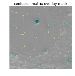
Now, let’s visualize and see where the confusion matrix elements TP, FP, FN, TN are distributed along the image. It shows us where the threshold is picking up foreground (vessels) when they are not present (FP) and where true vessels are not detected (FN), and vice-versa.
Validation visualization
To visualize confusion matrix elements, we figure out exactly where in the image the confusion matrix elements fall. For example, we find the TP array (i.e. pixels correctly detected as foreground) is by finding the logical “and” of the ground truth and the predicted array. Similarly, we use logical boolean operations commonly called as Bit blit to find the FP, FN, TN arrays.
get_confusion_matrix_intersection_mats()
def get_confusion_matrix_intersection_mats(groundtruth, predicted):

    """ Returns dict of 4 boolean numpy arrays with True at TP, FP, FN, TN

    """


    confusion_matrix_arrs = {}


    groundtruth_inverse = np.logical_not(groundtruth)

    predicted_inverse = np.logical_not(predicted)


    confusion_matrix_arrs['tp'] = np.logical_and(groundtruth, predicted)

    confusion_matrix_arrs['tn'] = np.logical_and(groundtruth_inverse, predicted_inverse)

    confusion_matrix_arrs['fp'] = np.logical_and(groundtruth_inverse, predicted)

    confusion_matrix_arrs['fn'] = np.logical_and(groundtruth, predicted_inverse)


    return confusion_matrix_arrs
Then, we can map pixels in each of these arrays to different colors. For the figure below we mapped TP, FP, FN, TN to the CMYK (Cyan, Magenta, Yellow, Black) space. One could similarly also map them to (Green, Red, Red, Green) colors. We would then get an image where everything in red signifies the incorrect predictions. The CMYK space allows us to distinguish between TP, TN.
get_confusion_matrix_overlaid_mask()
def get_confusion_matrix_overlaid_mask(image, groundtruth, predicted, alpha, colors):

    """

    Returns overlay the 'image' with a color mask where TP, FP, FN, TN are

    each a color given by the 'colors' dictionary

    """

    image = cv2.cvtColor(image, cv2.COLOR_GRAY2RGB)

    masks = get_confusion_matrix_intersection_mats(groundtruth, predicted)

    color_mask = np.zeros_like(image)

    for label, mask in masks.items():

        color = colors[label]

        mask_rgb = np.zeros_like(image)

        mask_rgb[mask != 0] = color

        color_mask += mask_rgb

    return cv2.addWeighted(image, alpha, color_mask, 1 - alpha, 0)


alpha = 0.5

confusion_matrix_colors = {

   'tp': (0, 255, 255),  #cyan

   'fp': (255, 0, 255),  #magenta

   'fn': (255, 255, 0),  #yellow

   'tn': (0, 0, 0)     #black

   }

validation_mask = get_confusion_matrix_overlaid_mask(255 - grayscale, groundtruth, predicted, alpha, confusion_matrix_colors)

print('Cyan - TP')

print('Magenta - FP')

print('Yellow - FN')

print('Black - TN')

plt.imshow(validation_mask)

plt.axis('off')

plt.title('confusion matrix overlay mask')
We use opencv here to overlay this color mask onto the original (non-inverted) grayscale image as a transparent layer. This is called Alpha compositing:
Final notes
The last two examples in the repository are testing the edge cases and a random prediction scenario on a small array (fewer than 10 elements), by calling the test functions. It is important to test for edge cases and potential issues if we are writing production level code, or just to test the simple logic of an algorithm.
Travis CI is very useful for testing whether your code works on the module versions described in your requirements, and if all the tests pass as new changes are merged into master. Keeping your code clean, well documented, and with all statements unit tested and covered is a best practice. These habits limit the need to chase down bugs, when a complex algorithm is built on top of simple functional pieces that could have been unit tested. Generally, documentation and unit testing helps others stay informed about your intentions for a function. Linting helps improve readability of the code, and flake8 is good Python package for that.
Here are the important takeaways from this article:
- Tiling and stitching approach for data that doesn’t fit in memory
- Trying different thresholding techniques
- Subtleties of Validation Metrics
- Validation visualization
- Best Practices
There are many directions you could go from here with your work or projects. Applying the same strategy to different data sets, or automating the validation selection approach would be excellent places to start. Further, imagine you needed to analyze a database with many of these 10gb files. How could you automate the process? How could you validate and justify the results to human beings? How does better analysis improve the outcomes of real-world scenarios (like the development of surgical procedures and medicine)? Asking questions like these will allow continued improvements in Statistics, Data Science, and Machine Learning.
Finally, Thanks to Navid Farahani for annotations, Katherine Scott for the guidance, Allen Teplitsky for the motivation, and all of the 3Scan team for the data.
Resources
 in San Francisco

