Python, NLTK, and the Digital Humanities: Finding Patterns in Gothic Literature
If someone says “gothic” to you, do you think of the lush rolling countryside or a sunny day?
Chances are you don’t. Most people – myself included – associate that word with the dark, mysterious, and even frightening. Maybe you picture ornate stone architecture of a castle with gargoyles. Or perhaps foreboding skies rolling over said castle. Or very morose, pale people wearing black capes and veils. Or vampires with all of the above.
About a year ago, Caroline Winter, a PhD student at the University of Victoria, emailed me with a question. She had assembled a corpus of 134 works of European Gothic literature that had been written or translated into English, ranging from the 18th century to the early 20th. Caroline had a hunch that gothic literature was more vibrant than most people thought, but lacked the quantitative background to analyze her large data set. Could I write a short script to count and analyze color words within her corpus? This post details my first experience with the digital humanities — applying simple computational tools programmers use every day to the data relevant to traditional humanities disciplines.
Originally a quick Python project for a Sunday afternoon, my journey attempting to answer Caroline’s question eventually turned into a talk at PyCon. Through some pretty straightforward counting and matching techniques, we were able to find several interesting patterns that challenged my gloomy picture of “gothic”. To follow along using Phantom of the Opera as an example text, take a look at the companion Jupyter Notebook on Github.
Beyond black & white
The first step in the project was to define which color words we were looking for. The challenge here was that both the vocabulary used to describe color and the actual coloring of objects themselves were different in the gothic era than in present day.
Rather than guess about historical color words, we turned to the Oxford English Dictionary’s Historical Thesaurus (hereafter the Historical Thesaurus). It lists color words used in English and primarily in Europe, the year of each one’s first recorded use, and its color family.
After adding some html color names based on color grouping to our csv file of the original data set I read a csv file with the Historical Thesaurus data into a short function and eliminated everything that came into usage after 1914, since it’s not clear from the data when words fell out of usage.
def id_color_words():

    """

    Gets color words from the csv file and puts them into a dict where key = word

    and value = (hex value, color family); removes pre-1914 color words.

    """

    color_word_dict = {}

    modern_color_words = []

    color_data = csv.DictReader(open('./color_names.csv'), delimiter=",", quotechar='"')


    for row in color_data:

        name = row['Colour Name'].lower()

        year = int(row['First Usage'])

        if ' ' not in name:

            if year < 1914:

                family = row['Colour Family'].lower()

                hex_value = row['hex'].lower()

                color_word_dict[name] = (hex_value, family)

            else:

                modern_color_words.append((year, name))


    return color_word_dict, modern_color_words
This gave us a dictionary of 980 pre-WWI color words ranging from the familiar, like blue (first usage in 1300), crimson (1416), or jet (1607), to the uncommon, like corbeau (1810, dark green), damask (1598, pink) or ochroid (1897, pale yellow). There were also some instances where the way words were categorized reflected a historical state of familiar things. For example, ‘glass’ is categorized as a greyish green, not pale blue or clear as we may think of it today.
Now we knew what we were looking for, but generating an accurate analysis was about more than simply counting these color words.
‘rose’ != ‘rose’ != ‘rose’
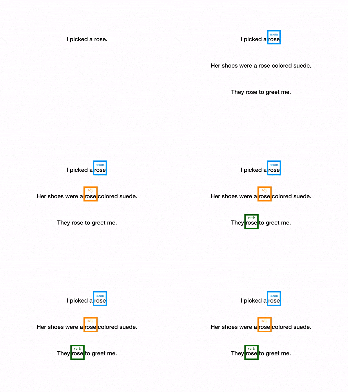
English is a tricky language, with many words that sound the same meaning different things and many words that look the same meaning different things depending on their context. ‘Rose’ is a great example: it can be a noun, adjective, or verb, as demonstrated in the gif below.

So which words should we count? Should every word on the list be included?
To make this decision, we needed to write more code to parse our corpus and look at the results.
I used the function below to get the text ready for analysis. It does three things. First, it reads in the .txt file for the work we’re analyzing. Then, the function removes the “gristle” of stop words, punctuation, and upper case letters. Finally, it leverages the pos_tag function from the Natural Language Toolkit (NLTK) to tag each remaining word as a part of speech (noun, verb, adjective, etc.).
def process_text(filename):

    """

    This function generates a list of tokens with punctuation stopwords, and spaces removed for the whole text.

    It also applies NLTK's part of speech tagging function to determine if words are nouns, adjectives, verbs, etc.

    """

    text_tokens = []


    # create a list of the words and punctuation we want to remove before analyzing

    stop_punc = set(stopwords.words('english') + [*string.punctuation] + ["''", '``'])


    with open(filename) as text:

        for row in text:

            # puts everything in lowercase, postion tags

            for token in pos_tag(word_tokenize(row.lower())):

                #removes tokens if contains punctuation or stopwords

                if token and token[0] not in stop_punc:

                    text_tokens.append(token)


    return text_tokens
This function outputs the whole text that looks like this – as you can see the NLTK pos_tag doesn’t look like it gets the part of speech correct every time, but it’s pretty close.
[('dying', 'JJ'),
('injunction', 'NN'),
('forbidden', 'VBN'),
('uncle', 'NN'),
('allow', 'VB'),
('embark', 'VB'),
('seafaring', 'JJ'),
('life', 'NN'),
('visions', 'NNS'),
('faded', 'VBD'),
('perused', 'VBD'),
('first', 'JJ'),
('time', 'NN'),
('poets', 'NNS'),
('whose', 'WP$'),
('effusions', 'NNS'),
('entranced', 'VBD'),
('soul', 'NN'),
('lifted', 'VBD'),
('heaven', 'VB')]
Next, we needed to isolate the color words from the text and do some analysis of the context to make sure there weren’t any glaring issues in the data we were generating. Here Caroline’s literature background was extremely helpful in identifying what looked inaccurate, and I went off to pull out the context of the suspicious words so she could make a final call.
- Isabella, a yellowish color that was also the name of a couple of characters in our corpus;
- Imperial, a purple color that in the texts actually meant the political structure, not the color; and
- Angry, sometimes used to describe a red-pink flushed color, but was used more often as an emotion word than a color word.
At this stage, I also experimented with stemming and lemmatizing the color words in our master list and in the texts themselves to see if that changed how many color words we were finding, rather than looking for exact matches. What this means, for example, is transforming the word “whitish” from the Historical Thesaurus to its root, or stem (“white”), and doing the same to the words in the text we were analyzing. However, because the Historical Thesaurus is so comprehensive and already included many forms of each word, the results didn’t change much and we decided to leave this step out.
Looking at the preliminary data, we also found that we got some combinations of color words, like “rose” followed by “red” or “milky” followed by “white”. While the Historical Thesaurus covers common combinations of these when they’re joined with a “-” (e.g. “rose-red”) we decided to isolate those examples in the output of the find_color_words to help us determine if we wanted to exclude those samples from the final analysis.
Analysis & Visualization – the (really) fun part
With adjustments made to the color word list, we can run the tagged text through the find_color_wordsfunction below and see both the concurrent color words and the full list. To do this, the code below leverages Python’s itertools with a couple of helper functions: pairwise and is_color_word.
def pairwise(iterable):

    """

    Returns a zip object, consisting of tuple pairs of words where the second word of tuple #1

    will be the first word of tuple #2, e.g. [('room', 'NN'), ('perfume', 'NN'),  ('lady', 'NN'), ('black', 'JJ')]

    from our `processed` variable becomes:

        [(('room', 'NN'), ('perfume', 'NN'))

        (('perfume', 'NN'), ('lady', 'NN'))

        (('lady', 'NN'), ('black', 'JJ'))

        (('black', 'JJ'), ('contents', 'NNS')]

    """

    a, b = tee(iterable)

    next(b, None)

    return zip(a, b)


def is_color_word(word, color_dict):

    """

    Compares at each word, tag tuple in `processed` to both the color dict and the allowed tags

    for adjectives and nouns

    """

    color, tag = word

    tags = {'JJ', 'NN'} # JJ = adjectives, NN = nouns

    return tag in tags and color in color_dict


def find_color_words(t, color_dict):

    """

    Leverages the previous two functions to identify the color words in the text and look for concurrent

    color words (e.g. 'white marble'), then returns each in a separate list.

    """

    color_words = []

    concurrent_color_words = []


    for o in t:

        if is_color_word(o, color_dict):

            color_words.append(o)


    for p, n in pairwise(t):

        if is_color_word(p, color_dict) and is_color_word(n, color_dict):

            concurrent_color_words.append((p, n))


    return color_words, concurrent_color_words
Here’s what we get from this function.
First, a list of all of the identified color words in the text and their tag, like this:
[('yellow', 'JJ'),
('black', 'JJ'),
('mourning', 'NN'),
('rose-red', 'JJ'),
('lily-white', 'JJ'),
('black', 'JJ'),
('black', 'JJ'),
('black', 'JJ'),
('white', 'JJ'),
('yellow', 'NN'),
('plum', 'NN'),
('glass', 'NN'),
('red', 'JJ'),
('coral', 'JJ'),
('pink', 'NN'),
('iron', 'NN'),
('glass', 'NN'),
('pink', 'JJ'),
('candid', 'JJ'),
('blue', 'JJ')]
Second, we get a list of tuples containing the color words that were adjectives or nouns closely followed by another adjective or noun in the original text. From The Phantom of the Opera, we get examples like:
(('glass', 'NN'), ('champagne', 'NN'))
(('pink', 'NN'), ('white', 'JJ'))
(('gold', 'NN'), ('purple', 'NN'))
(('water', 'NN'), ('bluey', 'NN'))
In most cases we didn’t think one of these took anything away from or obscured the other; in fact their close association often painted a clearer picture of color texture. So we left both words in.
From this you can get some summary stats, like what percentage of all uncommon words in the text were color words (Phantom is 0.9%), and what proportion are nouns versus adjectives (Phantom is 52-47).
But the really fun part is using those HTML color groups to plot the use of color in the text.
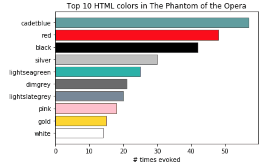
The Jupyter Notebook contains a couple of examples with matplotlib that are really straightforward to implement, like this bar chart showing the colors used in The Phantom of the Opera. Kite created a Github repository here where you can access the code from this and other posts on their blog.

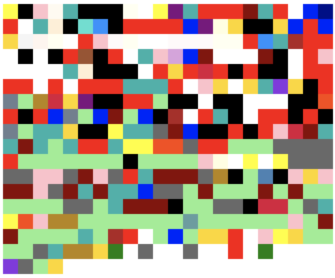
There are many of interesting options for visualizing this data. The original talk included a website, built with the Django framework, ChartJS, and lots of CSS – online here – where we visualized each book as a series of color blocks in their order of appearance.

Even with the limitations of HTML color applied to a broad palette, you’ll see that a lot of the books are not as dark and gloomy as their “gothic” label might lead you to believe. This makes sense: the supernatural is a strong theme in Gothic literature, but so is contrasting it with the beauty of the natural world that was considered both a haven and a dwindling reality during the dawn of the industrial revolution.
Beyond this post
Our talk at PyCon in 2017 was by no means the end of the project. A few months later, we were contacted by a scholar who used some of our color palettes for his research, and Caroline is in the process of writing up and publishing our findings. This will be one of the few explorations of color in gothic literature and, as far as we know, the only quantitative study on the topic. The project also inspired her to take a course in Python.
There are so many ways in which computing could be used for humanities scholarship to complement the strong traditions already there. I hope this project helps programmers and researchers alike consider the vast potential of the digital humanities. If you’d like to learn more about this project after reviewing, please watch the original talk and visit the website, check out the repo and the (extensive) corpus. If you prefer to work with more recent literature, check out my 2018 project where I explain and quantify gender bias in the Harry Potter series using Python.
This post is a part of Kite’s new series on Python. You can check out the code from this and other posts on our GitHub repository.
Resources
 in San Francisco

